One of the research projects I have been working on concerns mathematical reasoning and extrapolation on out-of-distribution (OOD) data in neural networks. Extrapolation is the ability of a model to correctly predict the output when given data sampled outside the training distribution. For example, if a model is trained on a ranger $[0,5]$ a valid OOD range may be something like $[6,10]$. Or, in the context of mathematical reasoning, we may train a model on some synthetic dataset based on some underlying algebraic rules, and then study in what sense a model may extrapolate on OOD data. We can ask questions like: is the model taking a statistical shortcut to predict results, or has it actually learned the algebraic rules? In other words, extrapolation means that the model successfully learns the underlying principles for modelling the mathematical operations (e.g., algebraic or arithmetic) it was trained on. These are the sort of questions my current research encircles: it concerns the conditions under which neural networks can perform mathematical computations beyond the distributions encountered during training.
Scientifically, there is an important distinction between a neural network, trained on finitely many examples of symbolic mathematical expressions, learning reusable computational rules that generalise beyond the training distribution, and merely exploiting statistical regularities or shortcuts that happen to predict the correct answer. Successful prediction does not necessarily imply that a network has acquired a systematic mathematical procedure. A model might achieve high OOD accuracy on particular symbolic benchmarks while exhibiting systematic failures on relatively simple expressions constructed differently from its training examples. Understanding such behaviour requires studying not only predictive performance, but also the computational representations and mechanisms supporting it.
In my opinion, this is one of the most interesting and highly debated areas of modern ML research. This is because, although neural networks have demonstrated impressive performance on various symbolic reasoning tasks, interpreting these results remains a significant challenge. In particular, strong predictive performance does not necessarily reveal the internal computational mechanisms responsible for generalisation, or establish their robustness under systematically different distributions. There are so many open questions about what is actually being represented internally, and when apparent mathematical competence collapses into superficial pattern matching, that I am hesitant to place my confidence in any research papers that currently claim to be conclusive.
In one of my projects, current experiments use a conventional character-level Gated Recurrent Unit (GRUs), starting with a single recurrent layer. (I am also working with a family of neural networks called Neural Arithmetic Logic Modules (NALMs), but we’ll talk about these in a separate entry). Although relatively simple compared with Transformers or other modern architectures equipped with explicit structural memory, the GRU is very useful experimental architecture for a number of reasons. To give some examples: its architectural constraints are well defined and it provides considerable control over the learning problem. Its recurrent hidden states can also be inspected to investigate how information is represented and transformed. More generally, this provides a controlled setting for studying finer details about how neural networks acquire reusable computational representations, and how these representations behave when things like sequence length, compositional structure, or mathematical complexity changes.
From basic recurrent neural networks to gated memory
What, then, is a GRU?
GRUs were introduced by Cho et al. in 2014 as a gated recurrent architecture for modelling sequences. Typically, as organised in most contemporary textbooks, one is introduced to GRUs directly after learning about long short-term memory (LSTM) models. Both LSTMs and GRUs are examples of recurrent neural networks (RNNs). Unlike a conventional or vanilla RNN, which repeatedly transforms its hidden state through a non-linear recurrence, an LSTM introduces a separate cell state together with multiplicative gates that regulate how information is incorporated, retained, and exposed. These gates were designed to help mitigate the difficulties conventional RNNs encounter when learning long-range dependencies.
The governing equations of an LSTM are fairly straightforward. Assuming there are ℎ hidden units with the batch size 𝑛, and with \(d\) number of inputs, define the input as \(X_t \in \mathbb{R}^{n\times d}\) and the hidden state of the previous time step \(H_{t-1} \in \mathbb{R}^{n\times h}\). The gates at time step 𝑡 are defined as follows: the input gate is \(I_t \in \mathbb{R}^{n\times h}\), the forget gate is \(F_t \in \mathbb{R}^{n\times h}\), and the output gate is \(O_t \in \mathbb{R}^{n\times h}\). It follows
\(I_t = \sigma(X_t W_{xi} + H_{t −1} W_{hi} + b_i),\) \(F_t = \sigma (X_t W_{xf} + H_{t-1}W_{hf} + b_f),\) \(O_t = \sigma (X_t W_{xo} + H_{t-1} W_{ho} + b_o) ,\)
where \(W_{xi}, W_{xf}, W_{xo} \in \mathbb{R}^{d \times h}\) and \(W_{hi}, W_{hf}, W_{ho} \in \mathbb{R}^{h \times h}\) are weight matrices, and \(b_i, b_f, b_o \in \mathbb{R}^{1 \times h}\) are bias vectors broadcast across the batch. The input node \(\tilde{C} \in \mathbb{R}^{n \times h}\) uses the \(\tanh\) function with a value range \(-1,1\) as the activation function. The activation function maps the gate activations into the interval \((0,1)\), with the gates themselves acting as continuous, differentiable controls over information flow, rather than exact binary switches.
For time \(t\), the candidate cell is given by
\[\tilde{C}_t = \tanh (X_t W_{xc}n+ H_{t-1}W_{hc} + b_c,\]where \(W_{xc}\in\mathbb R^{d\times h}\), \(W_{hc}\in\mathbb R^{h\times h}\), and \(b_c\in\mathbb R^{1\times h}\). Because \(\tanh\) maps real-valued inputs into \((-1,1)\), the candidate cell-state values are bounded within this interval.
When we include a hidden state, schematically we have a network as pictured below:
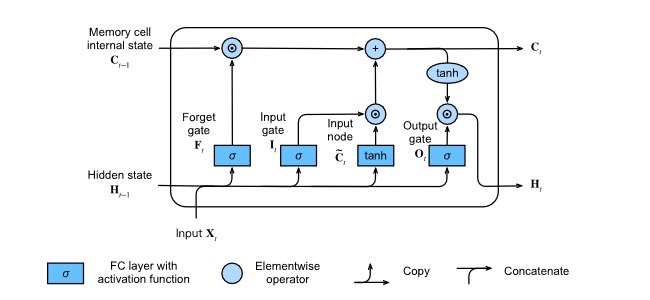
Computing the hidden state in an LSTM model. Borrowed from Dive into Deep Learning by Zhang et al.
There are two interesting features of an LSTM which, in many ways, help motivate the idea of a GRU. Using the Hadamard product, the memory cell internal state is given by the additive update
\(C_t = F_t \odot C_{t-1} + I_t \odot \tilde{C}_t\),
where the input gate (I_t) governs the quantity of new data inputed via \(\tilde{C}t\), and the forget gate governs how much is retained of the old cell internal state \(C_{t-1} \in \mathbb{R}^{n \times h}\). In practice, the input gate controls the contribution of the candidate cell state, the forget gate controls retention of the previous cell state, and the output gate controls how much of the transformed cell state is exposed through the hidden state. This matters because gating provides a learned, differentiable mechanism for controlling memory rather than an explicit system of discrete logical instructions.
The hidden state, \(H_t \in \mathbb{R}^{n \times h}\) is seen by the output after the \(\tanh\) function is applied such that
\[H_t = O_t \odot \tanh(C_t).\]This seemingly simple equation is actually very important. The central architectural innovation is the additive memory pathway
\[C_t= F_t\odot C_{t-1}+I_t\odot\tilde C_t.\]The cell state provides a separate memory pathway whose previous contents can be retained approximately unchanged when the forget gate approaches one. The exposed hidden state, by contrast, is regulated by the output gate and a non-linear transformation of the cell state. This additive memory pathway helps explain why LSTMs can mitigate some of the vanishing-gradient difficulties associated with conventional RNNs. Along the direct cell-state pathway, the contribution of the previous state is multiplied by the forget gate
\[\left.\frac{\partial C_t}{\partial C_{t-1}}\right|_{\text{direct}}=F_t.\]When \(F_t\) remains close to one, this pathway can preserve information and support gradient propagation across many time steps. This does not eliminate vanishing gradients altogether, since the complete recurrent derivatives also involve the dependence of the gates on previous states. Nevertheless, the additive cell-state mechanism provides an important architectural distinction from a vanilla RNN, and was central to the motivation for LSTMs in Hochreiter and Schmidhuber (1997). (The forget gate used in the modern LSTM formulation was introduced subsequently by Gers and colleagues).
Another interesting implication is that the LSTM cell state is not constrained to the interval \([-1,1]\) by a convex-combination update. Although the candidate state is bounded by \(\tanh\), repeated additive updates can produce cell-state magnitudes greater than one.
This distinction will become relevant when considering the recurrent state of a GRU.
The GRU: a simpler gated recurrent architecture
When it comes to GRUs, we basically have a much more streamlined version of an LSTM, achieving comparable performance and with the advantage of faster compute in certain applications. For comparable input and hidden dimensions, a conventional GRU uses three affine transformations for its reset, update and candidate computations, whereas a conventional LSTM uses four for its three gates and candidate cell state. By eliminating the LSTM’s separate cell state and reducing the number of gates from three to two, this generally reduces the number of parameters for comparable hidden dimensions, while retaining mechanisms for controlling information retention and state updates. Given an input sequence \(x_1,\ldots,x_T\), a GRU processes each element sequentially, updating a hidden representation according to a recurrence of the form
\[h_t = \mathcal{F}\theta (x_t, h_{t-1}),\]where \(h_t\) is the hidden state at time \(t\), and \(\mathcal{F}_\theta\) is a learned state-transition function whose parameters are shared across time steps. The important characteristic is that the dimensionality of \(h_t\) does not increase with the length of the input. The network repeatedly applied a learned transformation to a representation of fixed width.
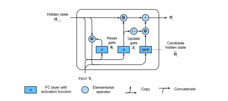
A GRU uses two gates to regulate its recurrent computation: the reset gate \(r_t\) and the update gate \(z_t\). (For clarity, we now use lowercase notation to describe a single sequence, rather than the batched matrix notation used in the LSTM equations above). The equations implemented by PyTorch’s nn.GRU are
\(r_t = \sigma(W_{ir}x_t+b_{ir} +W_{hr}h_{t-1}+b_{hr}),\) \(z_t = \sigma(W_{iz}x_t+b_{iz} +W_{hz}h_{t-1}+b_{hz}),\) \(n_t = \tanh\left(W_{in}x_t+b_{in} +r_t\odot(W_{hn}h_{t-1}+b_{hn})\right),\) \(h_t = (1-z_t)\odot n_t+z_t\odot h_{t-1},\)
where \(\sigma)\) is the sigmoid function and \(n_t\) is the candidate hidden state. The reset and update gates perform distinct, complementary functions. The reset gate regulates how the previous hidden state contributes to constructing the candidate state. The update gate determines the interpolation between the previous hidden state and the new candidate. For example, when a component of \(z_t\) approaches one, the corresponding component of the previous state is retained approximately unchanged. When it approaches zero, the candidate state contributes more strongly.
The reset gate, meanwhile, controls how much previous information participates in the candidate-state computation. Importantly, a reset gate close to zero does not automatically erase the previous hidden state, since the update gate may still preserve it in the final recurrence. But we’ll get to the hidden state in a moment.
The candidate-state equation in PyTorch differs from the formulation commonly presented in textbooks, such as Zhang et al.’s Dive into Deep Learning. In the textbook formulation, written using column vectors, the candidate state is
\[\tilde h_t= \tanh\left( W_{in}x_t+b_{in} +W_{hn}(r_t\odot h_{t-1})+b_{hn}\right).\]In PyTorch’s formulation, the corresponding calculation takes the form \(n_t= \tanh\left(W_{in}x_t+b_{in}+r_t\odot(W_{hn}h_{t-1}+b_{hn}) \right).\)
What’s different? Notice that in the first formulation, the rest gate acts on the previous hidden state before the hidden-to-hidden affine transformation. In PyTorch, it acts on the transformed recurrent contribution instead. These operations are not equivalent in general \(W(r\odot h)\neq r\odot(Wh)\). The implication of this is actually quite interesting. Gating before matrix multiplication changes how individual previous state coordinates contribute to the candidate representation, whereas gating afterward controls the resulting transformed coordinates. PyTorch documents this ordering as an implementation choice motivated by computational efficiency. But it actually matters for mathematical reasoning insofar that, unlike a model explicitly provided with the abstract syntax tree of an expression, a character-level GRU receives a sequence of symbols and must learn which aspects of that sequence are relevant to subsequent computation. Whilst both formulations implement the same broad architectural principle: recurrent information is selectively incorporated into a candidate representation, while an update gate controls how much of the previous hidden state is preserved.
The gating equations impose an interesting mathematical constraint on the GRU hidden state. The sigmoid gates take values in ((0,1)), while the candidate hidden state produced by (\tanh) lies in ((-1,1)). Because the final hidden state is an elementwise convex combination of the previous hidden state and the candidate state, a GRU initialised with (h_0=0) satisfies
\[h_t \in [-1,1]^{D}\]for every time step, where \(D\) is the hidden-state dimension. If, for example, \(D = 11\), then the model’s recurrent representation would be confined to a bounded \(11\)-dimensional hypercube. This follows inductively from the recurrence: if a previous hidden-state coordinate lies in \([-1,1]\), its convex combination with a candidate coordinate in \((-1,1)\) must also lie in \([-1,1]\).
However, bounded activation magnitude should not be confused with an inability to represent arbitrarily many distinct values in ideal real arithmetic. Moreover, bounded continuous space can, mathematically, contain infinitely many distinguishable states. In practical neural computation, the relevant limitations involve finite numerical precision, the learnability of useful encodings, and their robustness across recurrent transitions.
It is also important that bounded activations do not imply inevitable saturation or information loss. When \(z_t\) approaches one, the GRU can approximately preserve selected components of its previous state. Its learned dynamics may therefore support stable information retention, as well as forgetting or transformation.
The resulting question is not merely how many numerical values a bounded recurrent state can represent, but whether the network can learn state transitions that preserve the information required for systematic symbolic computation. Some operations may admit compact recurrent representations, whereas others, especially those involving unfamiliar nesting structures or long-range dependencies, may require more demanding internal organisation. This has been especially pertinent in my research, and, I would say, this distinction becomes particularly interesting when considering extrapolation generally.
It’s all in the GRU: Numerical extrapolation and structural generalisation
In the context of my current research, a useful distinction arises between extrapolating numerical values and interpreting increasingly complex symbolic structures. Consider a GRU with a scalar regression head,
\[\hat y=w^\top h_T+b.\]Since every coordinate of \(h_T\) is bounded, its output satisfies
\[\mid \hat y \mid \leq \mid b \mid + \mid w \mid_1.\]For fixed finite parameters, this architecture cannot represent a scalar function whose output grows without bound over an unlimited input domain. This observation is one that is also deeply relevant in the study of Neural Arithmetic Logic Units (NALUs) introduced by Trask et al. (2018) and other neural arithmetic systems, which was designed to encourage systematic extrapolation beyond observed numerical ranges.
Yet the boundedness of the regression output does not imply that a GRU must fail immediately outside the numerical range encountered during training. It establishes a global limit on the magnitude of the output for fixed parameters, not a precise threshold at which extrapolation must break down. Nor does it imply an equivalent failure in a symbolic classification task.
For a linear classification head, say,
\[\ell=Wh_T+b, \qquad \hat\lambda(e)=\arg\max_k\ell_k,\]each class corresponds to a region of hidden-state space defined by linear inequalities between logits. These regions need not form compact geometric clusters. Nevertheless, the network must learn recurrent transformations that place the final hidden state on the correct side of the relevant decision boundaries. (A bounded output space does not imply that the computation required to produce the correct output has bounded structural complexity). Recognising well-formed expressions with arbitrarily deep nesting, for example, may require increasingly demanding intermediate information even when the final prediction is binary. What I have found so far is that this makes it important to distinguish length extrapolation, structural-depth extrapolation, compositional extrapolation, and extrapolation to previously unseen output values.
The work of Bhattamishra, Ahuja and Goyal (2020) provides a particularly interesting example: recurrent networks can generalise to substantially longer hierarchical sequences when nesting depth is bounded, while unrestricted hierarchical generalisation presents greater difficulties. This suggests that length extrapolation, structural-depth extrapolation, compositional extrapolation, and extrapolation to unseen output values should be treated as distinct experimental questions. Success in one regime does not necessarily imply success in another. Linear probes
One advantage of working with a small GRU for studies on generalisation and mathematical reasoning is that its hidden states can be inspected at every character position. This makes it possible to investigate whether the recurrent representation contains information about mathematical properties such as nesting depth, operator scope, intermediate cardinality levels, or partial expression structure.
For instance, a linear probe could be trained to predict a mathematical property from intermediate hidden states. Principal component analysis or other representational methods might reveal systematic geometric relationships between states associated with different expression structures.
Yet interpretability requires an important distinction between information being decodable from a representation and information being causally used by the network. A successful probe does not, by itself, establish that the model relies on the decoded property to make its prediction. Such analyses can establish the accessibility of task relevant information to a probe, but stronger mechanistic claims require additional evidence, potentially including controlled interventions on hidden representations and measurements of their effects on model predictions. A complementary question concerns the stability of recurrent computation over longer or unfamiliar sequences. Writing the recurrence as a composition of learned transitions,
\[h_T=F_{x_T}\circ\cdots\circ F_{x_1}(h_0),\]we can examine how small perturbations to an intermediate hidden state propagate through subsequent recurrent updates.
Define the Jacobian
\[J_s=\frac{\partial h_{s+1}}{\partial h_s},\]where the input sequence is held fixed, then, to first order,
\[\delta h_T\approx J_{T-1}J_{T-2}\cdots J_t,\delta h_t.\]Each \(J_t\) is the Jacobian of the recurrent transition with respect to the previous hidden state. Depending on the learned dynamics, perturbations may contract, expand, or remain relatively stable. This potentially gives a mathematical basis for studying information retention, sensitivity, and possible representational instability. However, recurrent computation does not inevitably produce representational drift. A learned state transition may be stable, may preserve task-relevant information, or may systematically lose information under particular conditions. The effect of longer sequence horizons therefore depends on the learned dynamics, not merely on the repeated application of recurrent updates. Furthermore, local Jacobian sensitivity does not, by itself, establish whether the network has learned a mathematically correct computational procedure. It characterises properties of the recurrent dynamics that can then be related to behavioural performance and the information encoded in hidden states. One thing I have been investigating is the connection between behavioural failures and measurements of the hidden-state dynamics, and ultimately the question on how to distinguish correlational patterns from causal mechanisms through controlled interventions.
These are some of the reasons I find the GRU to be a useful scientific tool. Their simplicity does not make them mathematically uninteresting; it makes the relationship between recurrent computation, learned structure, and generalisation particularly amenable to controlled empirical investigation. Although seemingly simplistic when compared against more popular contemporary architectures, a small GRU can be scientifically useful because the same gated state-transition mechanism processes every character; the model is not explicitly supplied with intermediate oracle values, symbolic parsing operations, or external structural memory. My broader interest is to understand the relationship between computational architecture, learned representation, and the systematic interpretation of mathematical structure. An important part of this investigation is to distinguish three levels of evidence: behavioural performance, the mathematical information represented internally, and the mechanisms through which that information influences computation. A key part of this research involves the progression from characterising the structural conditions under which a GRU generalises or fails, to investigating it hidden-state representations, and eventually to introducing controlled inerventions that test specific explanations for its behaviour.